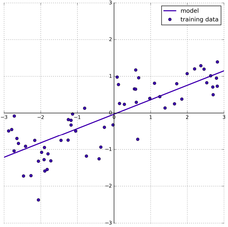
Linear regression, or ordinary least squares (OLS), is the simplest and most classic linear method for regression. Linear regression finds the parameters \(\Theta\) that minimize the mean squared error between predictions and the true regression targets, y, on the training set. The mean squared error is the sum of the squared differences between the predictions and the true values. Linear regression has no parameters which is a benefit, but is also has no way to control model complexity.

from sklearn.linear_model import LinearRegression
X, y = mglearn.datasets.make_wave(n_samples=60)
X_train, X_test, y_train, y_test = train_test_split(X, y, random_state=42)

lr = LinearRegression().fit(X_train, y_train)
The values of \(\Theta_i , i=1, ..., N\), also called weights or coefficients, are stored in the coef_ atribbute, while the offset or intercept (\(\Theta_0\)) is stored in the *intercept_ attribute:
In:
print("lr.coef_: {}".format(lr.coef_))
print("lr.intercept_: {}".format(lr.intercept_))
Out:
lr.coef_: [ 0.394]
lr.intercept_: -0.031804343026759746
Let’s look at the training set and test set performance:
In:
print("Training set score: {:.2f}".format(lr.score(X_train, y_train)))
print("Test set score: {:.2f}".format(lr.score(X_test, y_test)))
Out:
Training set score: 0.67
Test set score: 0.66
An \(R^2\) of around 0.66 is not very good, but we can see that the scores on the training and test sets are very close together. This means we are likely underfitting, not overfitting. For this one-dimensional dataset, there is little danger of overfitting, as the model is very simple. However, with higher-dimensional datasets, linear models become more powerful, and there is a higher chance of overfitting.
If there was a huge discrepancy between performance on the training data and the test data is a clear sign of overfitting, and therefore we should try to find a model that allows us to control complexity.