Naive Bayes Classifiers are a family of classifiers very similar to the linear models. However, they tend to be even faster in training. The price paid for this efficiency is that Naive Bayes models provide generalization performance slightly worse than that of linear classifiers like Logistic Regression and Linear SVC.
The reason why Naive Bayes models are so efficient is that they learn parameters by looking at each feature individually and collect simples per-class statistics from each feature. For example, a fruit may be considered to be an apple if it is red, round, and about 3 inches in diameter. Even if these features depend on each other or upon the existence of the other features, all of these properties independently contribute to the probability that this fruit is an apple and that is why it is known as ‘Naive’.
Bayes’Theorem
Bayes’Theorem finds the probability of an event occurring given the probability of another event that has already occured.
\[P(A \mid B) = \frac{ P(B \mid A)P(A)}{P(B)}\]- Basically, we are trying to find probability of event A, given the event B is true. Event B is also termed as evidence.
- \(P(A)\) is the priori of A (i.e. the probability of event before evidence is seen). The evidence is an attribute value of an unknown instance.
- \(P(A \mid B)\) is a posteriori probability of B, i.e the probabily of event after evidence is seen.
How Naive Bayes Works?
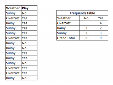
I have a training data set of weather and corresponding target ‘Play’. Now we need to classify whetever players will play or not based on weather condition. Example from Analytics Vidhya.
-
Step 1: Convert the data into a frequency table

-
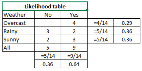
Step 2: Create Likehood table by finding the probabilities

-
Step 3: Now, use Naive Bayesian equation to calculate the posterior probability for each class. The class with highest probability is the outcome prediction.
Problem: Players will play if weather is sunny. This statement is correct?
\(P(Yes \mid Sunny) = \frac{P(Sunny \mid Yes)P(YES)}{P(Sunny)}\) \(P(Yes \mid Sunny) = \frac{\frac{3}{9} \cdot \frac{9}{14}}{\frac{5}{14}} = 0.60\text{, which is a higher probability}\)
Naive Bayes Classifiers Variants
There are three kinds of Naive Bayes classifiers: GuassianNV, BernoulliNB, and MultinomialNV. GuassianNB can be applied to any countinuous data, while BernoulliNV assumes binary data as MultinomailNB assumes count data (that is, each feature represents an integer count of something, like often a word appers in a sentence). BernoulliNB and MultinomialNB are mostly used in text data classification.
- Guassian it is used in classification and it assumes that features follow a normal distribution.
- Multinominal it is used for discrete counts. For example, let’s say, we have a text classification problem. Here we can consider Bernoulli trials which is one step further and instead of “word occurring in the document”, we have “count how often word occurs in the document”, you can think of as “number of times outcome number \(x_i\) is observed over the \(n\) trials”.
- Binomial the binomial model is useful if your feature vectores are binary. One application would be text classification, where the 1s and 0s are “word occurs in the document” and “word does not occur in the document” respectively.
To make prediction, a data point is compared to the statistics for each of the classes, and the best matching class is predicted. Interestingly, for both MultinomialNB and BernoulliNB, this leads to a prediction formula that is of the same form as in the linear models.
Strenghts, Weaknesses, and Parameters
MultinomialNB and BernoulliNB have a single parameter, alpha, which controls model complexity. The way alpha works is that the algorithm adds to the data alpha many virtual points that have positive values for all the features. This results in a “smoothing” of the statistics. A large alpha means more smoothing, resulting in less complex models. The algorithm’s performance is relatively robust to the setting of alpha, meaning that setting alpha is not critical for good performance. However, tuning it usually improves accuracy somewhat.
GuassianNB is mostly used on very high-dimensional data, while the other two variants of naive Bayes are widely used for sparse count data such as text. MultinominalNB usually performs better than BinaryNB, particulary on datasets with a relatively large number of nonzero features (i.e. large documents).
The Naive Bayes models share many of the strenghts and weaknesses of the linear models. They are very fast to train and to predict, and the training procedure is easy to understand. The models work very well with high-dimensional sparse data and are relatively robust to the parameters. Naive Bayes models are great baseline models and are often used on very large datasets, where training even a liner model might take too long.