Kernelized Support Vector Machines

Kernelized support vector machines (often just referred to as SVMs) are an extension that allows for more complex models that are not defined simply by hyperplanes in the input space. While there are support vector machines for classification and regression, we will restrict ourselves to the classification case, as implemented in SVC.

Linear Models and NonLinear Features

Linear Models can be quite limiting in low-dimensional spaces, as lines and hyperplanes have limited flexibility. One way to make a linear model more flexible is by adding more features - for example, by adding interactions or polynomials of the input features.

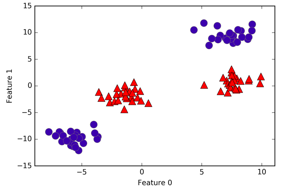
A linear model for classification can only separate points using a line, and will not be able to do a very good job on this dataset. Let’s now expanding the dataset dimension adding a new feature, as \((feature_1)^2\).

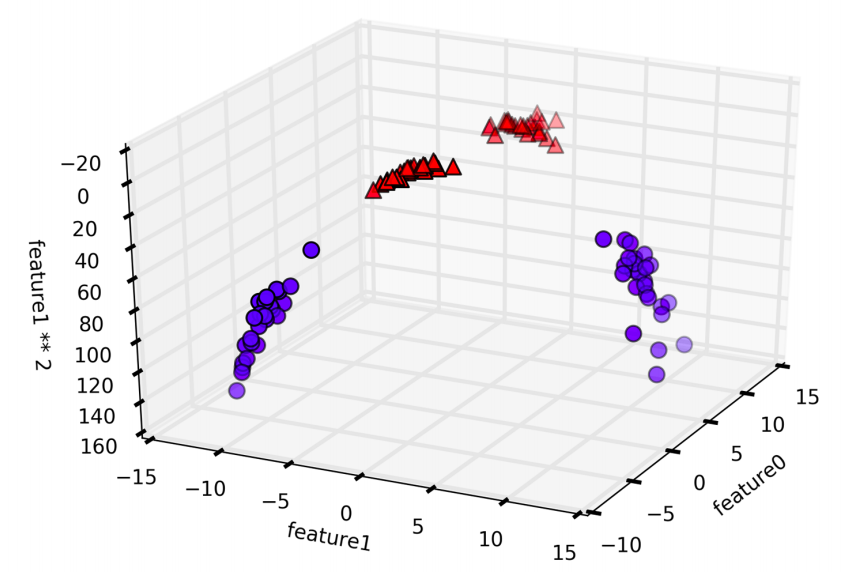
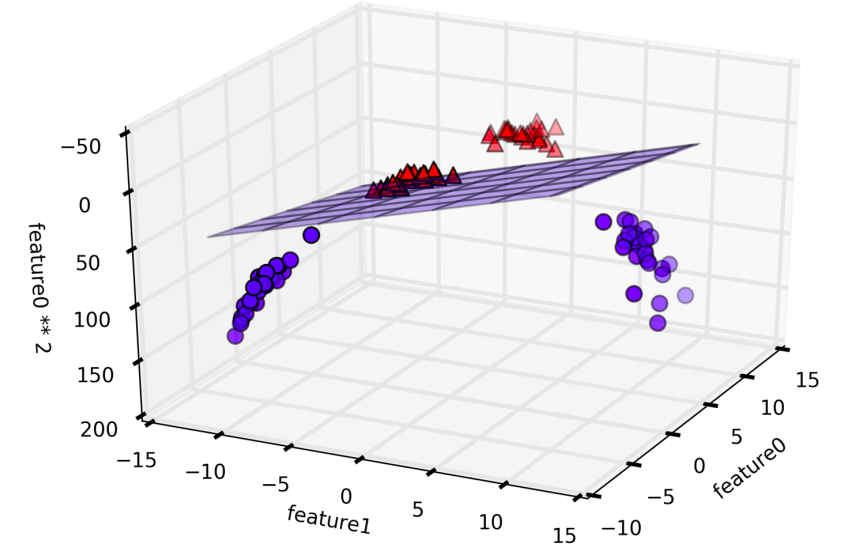
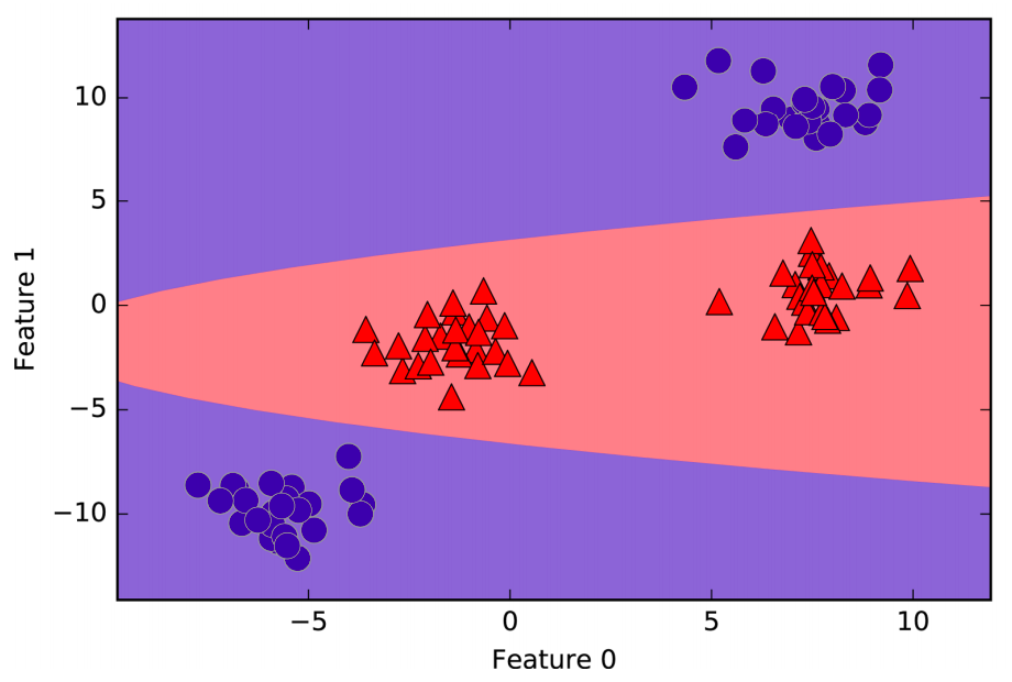
In the new representation of the data, it is now possible to separate the two classes using a linear model, through a plane. However, as a function of the original features, the linear SVM model is not actually linear anymore. It is not a line, but more of an ellipse.

The kernel trick

The lesson here is that adding nonlinear features to the representation of our data, it is possible make linear models much more powerful. However, often we don’t know which features to add, and adding many features might make computation very expensive. Luckily, there is a clever mathematical trick that allows us to learn a classifier in a higher-dimensional space without actually computing the new, possible very large representation. This is known as kernel trick, and it works by directly computing the distance (more precisely, the scalar products) of the data points for the expanded feature representation, without ever actually computing the expansion.

There are two ways to map your data into a higher-dimensional space that are commonly used with SVMs: the polynomial kernel, which computes all possible polynomials up to a certain degree of the original features; and the radial basis function (RBF) kernel, also known as the Guassian kernel.

Understanding SVMs

While training, the SVM learns how important each data point is important to represent the decision boundary between the two classes. Typically, only a subset of the training points matter for defining the decision boundary: the ones that lie on the border between classes. They are called support vectors and give the support vector machine its name.

To make a prediction for a new point, the distance to each of the support vectors is measured. A classification decision is made based on the distances to the support vector, and the importance of the support vectors that was learned during training. (stored in the dual_coef_attribute of SVC).

The distance between data points is measured by the Guassian kernel:

Here, \(x1\) e \(x2\) are data points, \(\|x1 - x2\|\) denotes Euclidean distance, and \(\gamma\) (gamma) is the parameter that controls the width of the Guassian kernel. Figure bellow shows the result of training a support vector machine on a twodimensional two-class dataset. The decision boundary is shown in black, and the support vectors are larger points with the wide outline.

In:
from sklearn.svm import SVC
X, y = mglearn.tools.make_handcrafted_dataset()
svm = SVC(kernel='rbf', C=10, gamma=0.1).fit(X, y)

mglearn.plots.plot_2d_separator(svm, X, eps=.5)
mglearn.discrete_scatter(X[:, 0], X[:, 1], y)

# plot support vectors
sv = svm.support_vectors_

# class labels of support vectors are given by 
# the sign of the dual coefficients
sv_labels = svm.dual_coef_.ravel() > 0
mglearn.discrete_scatter(sv[:, 0], sv[:, 1], sv_labels, 
    s=15, markeredgewidth=3)
plt.xlabel("Feature 0")
plt.ylabel("Feature 1")

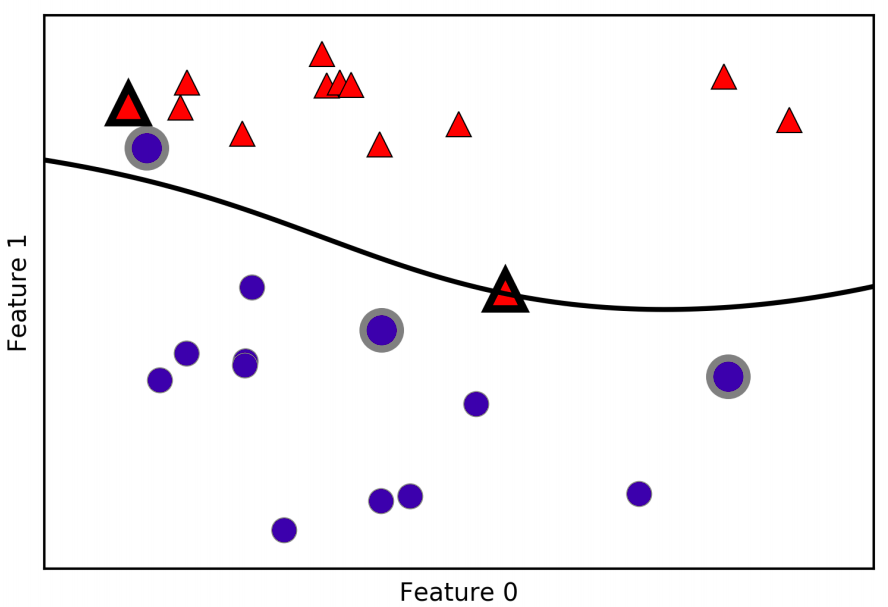
In this case, the SVM yields a very smooth and nonlinear (not a straight line) boundary. We adjusted two parameters here: the \(C\) parameter and the \(\gamma\) parameter.

Tunning SVM paramters

The \(\gamma\) parameter is the one that controls the width of the Guassian kernel. It determines the scale of what it means for points to be close together. The \(C\) paramter is a regularization parameter, similar to that used in the linear models. It limits the importance of each point.

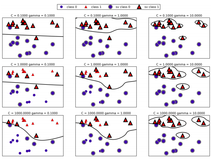
Going from left to right, we increase the value of the parameter \(\gamma\) from 0.1 to 10. A small gamma means a large radius for the Guassian kernel, which means that many points are considered close by. This is reflected in very smooth decision boundaries on the left, and boundaries that focus more on single points further to the right. A low value of gamma means that the decision boundary will vary very slow, which yields a model of low complexity, which a high value of gamma yields a more complex model.

Going from top to bottom, we increase the \(C\) parameter from 0.1 to 1000. As with the linear models, a small \(C\) means a very restricted model, where each data point can only have very limited influence. You can see that at the top left the decision boundary looks very nearly linear, with the misclassified points barely having any influence on the line. Increasing \(C\), as shown on the bottom right, allows these points to have a stronger influence on the model and makes the decision boundary bend to correctly classify them.

SVMs often perform quite well, they are very sensitive to the settings of the parameters and to the scalling of the data. In particular, they require all the features to vary on a similar scale.

Preprocessing data for SVMs

One way to resolve the scalling of the data is by rescaling each feature so that they are all approximately on the same scale. A common rescaling method for kernel SVMs it to scale the data such that all features are between 0 and 1, using the MaxMinScaler.

Strenghts, Weaknesses, and Parameters

Kernelized support vector machines are powerful models and perform well on a variety of datasets. SVMs allow for complex decision boundaries, even if the data has only a few features. They work well on low-dimensional and high-dimensional data, but don’t scale very well with the number of samples. Runing a SVM on data with up to 10,000 samples might work well, but working with datasets of size 100,000 or more can become challenging in terms of runtime and memory usage.

Another downside of SVMs is that they require careful preprocessing of the data and tuning of the parameters. This is why, these days, most of people instead use tree-based models such as random forests or gradient boosting (which require little or no preprocessing) in many applications. Furthermore, SVM models are hard to inspect; it can be dificult to understand why a particular prediction was made, and it might be tricky to explain the model to a nonexpert.

Still, it might be worth trying SVMs, particularly if all of your features represent measurements in similar units (e.g. all are pixel intensities) and they are on similar scales.

The important parameters in kernel SVMs are the regularization parameter \(C\), the choice of the kernel, and the kernel-specific parameters. Although we primarily focused on the RBF kernel. The RBF kernel has only one parameter, \(\gamma\), which is the inverse of the width of the Guassian kernel. \(\gamma\) and \(C\) both control the complexity of the model, with large values in either resulting in a more complex model. Therefore, good settings for the two parameters are usually strongly correlated, and \(C\) and \(\gamma\) should be adjusted together.