Neural Networks

While deep learning shows great proimise in many machine learning applications, deep learning algorithms are often tailored very carefully to be specific use case. Here, we will discuss some relatively simple methods, namely mutilayer perceptrons for classification and regression, that can serve as a starting point for more involved deep learning methods. Multilayer perceptrons (MLPs) are also known as (vanilla) feed-forward neural networks, or sometimes just neural networks.

Neural Network model

MPLs can be viewed as generalizations of linear models that perform mutiple stages of processing to come to a decision. A prediction by a linear model is given by:

The \(y\) is a weighted sum of the input features \(\theta\), weighted by the learned coefficients \(x\). In a MLP this process of computing weighted sums is repeated multiple times, first computing hidden units that represent an intermediate processing step, which are again combined using weighted sums to yield the final result.

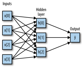
This model was a lot of coefficients (also called weights) to learn: there is one between every input and every hidden unit, and one between each hidden unit and the output node.

Computing a series of weighted sums is mathematically the same as computing just one weighted sum, so to take this model truly powerful than a linear model, we need one extra trick. After computing a weighted sum for each hidden unit, a nonlinear function is applied to the result - usually the rectifying nonlinearity (known as rectified linear unit or relu) or the tangens hyperbolicus (tanh). The result of this function is then used in the weighted sum that computes the output.

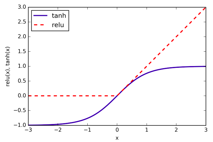
The relu cuts off values below zero, while tanh saturates to -1 for low input values and +1 for high input values. Either nonlinear functions allows the neural network to learn much more complicated functions than a linear model could.

For the small neural network pictured in Figure 2-45, the full formula for computing output in the case of regression would be (when using a tanh nonlinearity):

\(h[0] = tanh(\theta[0, 0] \cdot x[0] + \theta[1, 0] \cdot x[1] + \theta[2, 0] \cdot x[2] + \theta[3, 0] \cdot x[3])\) \(h[1] = tanh(\theta[0, 0] \cdot x[0] + \theta[1, 0] \cdot x[1] + \theta[2, 0] \cdot x[2] + \theta[3, 0] \cdot x[3])\) \(h[2] = tanh(\theta[0, 0] \cdot x[0] + \theta[1, 0] \cdot x[1] + \theta[2, 0] \cdot x[2] + \theta[3, 0] \cdot x[3])\) \(ŷ = v[0] \cdot h[0] + v[1] \cdot h[1] + v[2] \cdot h[2]\)

Here, \(\theta\) are the weights between the input \(x\) and the hidden layer \(h\), and \(v\) are the weights between the hidden layer \(h\) and the output \(ŷ\). The weights \(v\) and \(\theta\) are learned from data, \(x\) are the input features, \(ŷ\) is the computed output, and \(h\) are intermediate computations. An important parameter that needs to be set by the user is the number of nodes in the hidden layer. This can be as small as 10 very small or simple datasets and as big as 10,000 for very complex data. It is possible to add additional hidden layers.

Tuning Neural Networks

In:
from sklearn.neural_network import MLPClassifier
from sklearn.datasets import make_moons

X, y = make_moons(n_samples=100, noise=0.25, random_state=3)
X_train, X_test, y_train, y_test = train_test_split(X, y, stratify=y,
 random_state=42)

mlp = MLPClassifier(algorithm='l-bfgs', random_state=0)
 .fit(X_train, y_train)
mglearn.plots.plot_2d_separator(mlp, X_train, fill=True, alpha=.3)
mglearn.discrete_scatter(X_train[:, 0], X_train[:, 1], y_train)
plt.xlabel("Feature 0")
plt.ylabel("Feature 1")

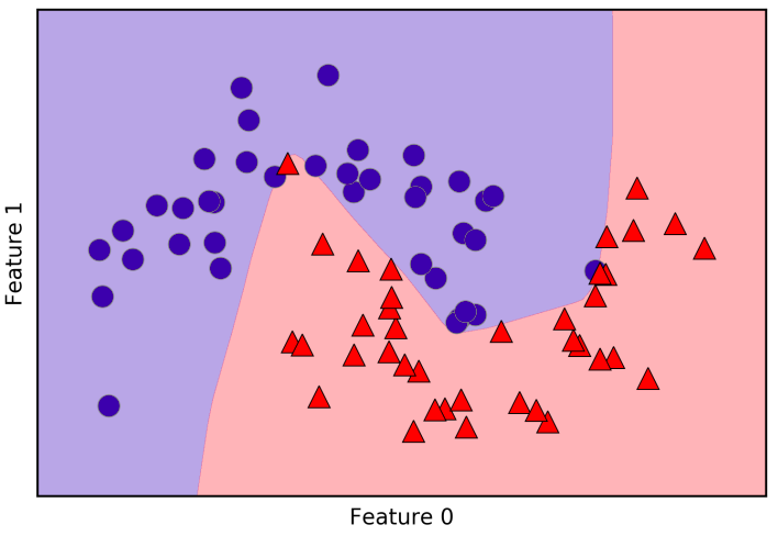
As is possible to see, the neural netwooks learned a very nonlinear but relatively smooth decision boundary. By default, the MLP uses 100 hidden layers, which is quite a lot for a small dataset. We can reduce the number (which reduce the complexity of the model) and still get a good result.

In:
mlp = MLPClassifier(algorithm='l-bfgs', random_state=0, 
    hidden_layer_sizes=[10]).fit(X_train, y_train)

mglearn.plots.plot_2d_separator(mlp, X_train, fill=True, alpha=.3)
mglearn.discrete_scatter(X_train[:, 0], X_train[:, 1], y_train)
plt.xlabel("Feature 0")
plt.ylabel("Feature 1")

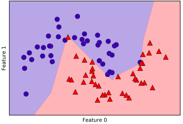
With only 10 units, the decision boundary looks somewhat more ragged. The default nonlinearity is relu. With a single layer, this means the decision boundary will be made up of 10 straight line segments. If we want a smoother decision boundary, we could add more hidden units.

Finally, we can also control de complexity of a neural network by using an l2 penalty to shrink the weights toward zero, as we did in ridge regression and the linear classifiers. The parameter for this in MLPClassifier is \(alpha\), and it’s set to a very low value (little regularization) by default. The figure below shows the effect of different values of \(alpha\) on the two_moons dataset, using two hidden layers of 10 or 100 units each.

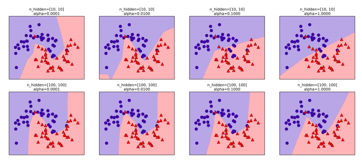
There are many ways to control the complexity of a neural network: the number of hidden layers, the number of units in each hidden layer, and the regularization (alpha). There are actually even more, which we won’t go into here.

An important property of neural networks is that their weights are set randomly before learning is started, and this random initialization affects the model that is learned. That means that even when using exactly the same parameters, we can obtain very different models when using different random seeds. If the networks are large, and their complexity is chosen properly, this should not affect accuracy too much, but it is worth keeping in mind (particularly for smaller networks).

Example

To get a better understanding of neural networks on real-world data, let’s apply the MPLClassifier to the a dataset called Breast Cancer. We start with the default parameters.

In:
X_train, X_test, y_train, y_test = train_test_split(
 cancer.data, cancer.target, random_state=0)

mlp = MLPClassifier(random_state=42)
mlp.fit(X_train, y_train)

print("Accuracy on training set: {:.2f}"
    .format(mlp.score(X_train, y_train)))
print("Accuracy on test set: {:.2f}"
    .format(mlp.score(X_test, y_test)))

Out:
Accuracy on training set: 0.92
Accuracy on test set: 0.90

The performance is quite good, but not good as the other models. As in the earlier SVC example, this is likely due to scaling of the data. Neural Networks also expect all input features to vary in a similar way, and ideally to have a mean of 0, and a variance of 1. We must rescale our data so that it fulfills these requirements.

In:
# compute the mean value per feature on the training set
mean_on_train = X_train.mean(axis=0)
# compute the standard deviation of each feature on the training set
std_on_train = X_train.std(axis=0)

# subtract the mean, and scale by inverse standard deviation
# afterward, mean=0 and std=1
X_train_scaled = (X_train - mean_on_train) / std_on_train
# use THE SAME transformation (using training mean and std) on the test set
X_test_scaled = (X_test - mean_on_train) / std_on_train

mlp = MLPClassifier(random_state=0)
mlp.fit(X_train_scaled, y_train)
print("Accuracy on training set: {:.3f}".format(
 mlp.score(X_train_scaled, y_train)))
print("Accuracy on test set: {:.3f}".format(
 mlp.score(X_test_scaled, y_test)))

Out:
Accuracy on training set: 0.991
Accuracy on test set: 0.965

ConvergenceWarning:
 Stochastic Optimizer: Maximum iterations reached and the optimization
 hasn't converged yet.

The results are much better after scalling, and already quite competitive. We got a warning from the model, through, that tells us that the maximum number of iterations has been reached. We should increase the number of iterations.

In:
mlp = MLPClassifier(max_iter=1000, random_state=0)
mlp.fit(X_train_scaled, y_train)

print("Accuracy on training set: {:.3f}".format(
 mlp.score(X_train_scaled, y_train)))
print("Accuracy on test set: {:.3f}".format(
 mlp.score(X_test_scaled, y_test)))

Out:
Accuracy on training set: 0.995
Accuracy on test set: 0.965

Increasing the number of iterations only increase the training set performance, not the generalization performance. Still, the model is performing quite well. As there is some gap between the training and the test set performance, we might try to decrease the model’s complexity to get better generalization performance. Here, we choose to increase the alpha parameter to add stronger regularization of the weights.

In:
mlp = MLPClassifier(max_iter=1000, alpha=1, random_state=0)
mlp.fit(X_train_scaled, y_train)

print("Accuracy on training set: {:.3f}".format(
 mlp.score(X_train_scaled, y_train)))
print("Accuracy on test set: {:.3f}".format(
 mlp.score(X_test_scaled, y_test)))

Out:
Accuracy on training set: 0.988
Accuracy on test set: 0.972

This leads to a performance on par with the best models so far. At this point that many of the well-performing models achieved exactly the same accuracy of 0.972. This means that all the models make exactly the same number of mistakes, which is four. This may be a consequence of the dataset being very small, or it may be because these points are really different from the rest.

While is possible to analyze what a neural networks has learned, this is usually much trickier than analyzing a linear model or a tree-based model. One way to introspect what was learnead is to look at weights in the model. For the Breast Cancer dataset, the dataset we were working on until now, the following plot shows the weights that were learned connecting the input to the first hidden layer. The rows in this plot correspond to the 30 input features, while the columns correspond to the 100 hidden units.

One possible inference we can make is that features that have very small weights for all of the hidden units are “less important” to the model. We can see that “mean smoothness” and “mean compactness”, in addition to the features found between “smoothness error” and “fractal dimension error”, have relatively low weights compared to other features. This could mean that these are less important features or possibly that we didn’t represent them in a way that the neural network could use.

We could also visualize the weights connecting the hidden layer to the output layer, but those are even harder to interpret.

Strenghts, Weaknesses, and Parameters

Neural networks have reemerged as state-of-the-art models in many applications of machine learning. One of their main advantages is that they are able to capture information contained in large amounts of data and build incredibly complex models. Given enough computation time, data, and careful tuning of the parameters, neural networks often beat other machine learning algorithms (for classification and regression tasks).

Unfortunally, neural networks - particularly the large and powerful ones - often take a long time to train. They also require carefull preprocessing of the data, as we saw here. Similarly to SVMs, they work best with “homogeneous” data, where all the features have similar meanings. For data that has very different kinds of features, tree-based models might work better. Tunning neural network parameters is also an art unto itself. In our experiments, we barely scratched the surface of possible ways to adjust neural network models and how to train them.

Estimating complexity in neural networks

The most important parameters are the number of layers and the number of hidden units per layer. You should start with one or two hidden layers, and possibly expand from there. The number of nodes per hidden layer is often similar to the number of input features, but rarely higher than in the low to mid-thousands.

A helpful measure when thinking about the model complexity of a neural network is the number of weights or coefficients that are learned. If you have a binary classification dataset with 100 features, and you have 100 hidden units, then there are \(100\cdot100 = 10,000\) weights between the input and the first hidden layer. There are also \(100\cdot1=100\) weights between the hidden layer and the output layer, for a total of around 10,100 weights. If we add a second hidden layer with 100 hidden units, there will be another \(100\cdot100 = 10,000\) weights from the first hidden layer to the second hidden layer, resulting in a total of 20,100 weights.

If instead you use one layer with 1,000 hidden units, you are learning \(100 \cdot 1,000 = 100,000\) weights from the input to the hidden layer and \(1,000 \cdot 1\) weights from the hidden layer to the output layer, for a total of 101,000. If you add a second hidden layer you add \(1,000 \cdot 1,000 = 1,000,000\) weights, for a whopping total of 1,101,000 - 50 times larger than the model with two hidden layers of size 100.

A common way to adjust parameters in a neural network is to first create a network that is large enough to overfit, making sure that the task can actually be learned by the network. Then, once you know the training data can be learned, either shrink the network or increase alpha to add regularization, which will improve generalization performance.

There is also the question of how to learn the model, or the algorithm that is used for learning the parameters, which is set using the algorithm parameter. There are two easy-to-use choices for algorithm. The default is ‘adam’, which works well in most situations but is quite sensitive to the scaling of the data. The other one is ‘l-bfgs’, which is quite robust but might take a long time on larger models or larger datasets. There is also the more advanced ‘sgd’ option, which is what many deep learnings researches use. The ‘sgd’ option comes with manu addition parameters that need to be tuned for best results.