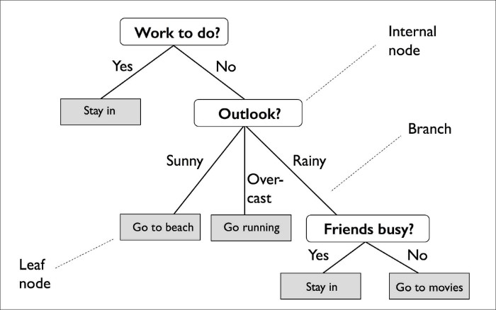
Decision trees are widely used models for classification and regression tasks. Essentially, they predict a target by learning decision rules from features. As the name suggests, we can think of this model as breaking down our data by making a decision based on asking a series of questions.

Based on the features in our training set, the decision tree model learns a series of questions to infer the class labels of the samples. As we can see, decision trees are attractive models if we care about interpretability.
A decision tree is constructed by recursive partioning - starting from a root node (called first parent), and each node can be split into left and right child nodes. Nodes that do not have any child are known as terminal/leaf nodes.
A decision tree makes decisions by splitting nodes into sub-nodes. This process is performed multiple times during the training process until only homogenous nodes are left. Node splitting, or splitting, is the process of dividing a node into multiple sub-nodes to create relatively terminal nodes. There are multiple ways of doing this, which can be broadly divided into two categories based on the type of target variable:
- Continuous target variable
- Reduction in Variance
- Categorical target variable
- Gini Impurity
- Entropy/Information Gain
- Chi-Square
Although the preceding figure illustrates the concept of a decision tree based on categorical targets (classification), the same concept applies if our targets are real numbers (regression).
Controlling complexity of decision trees
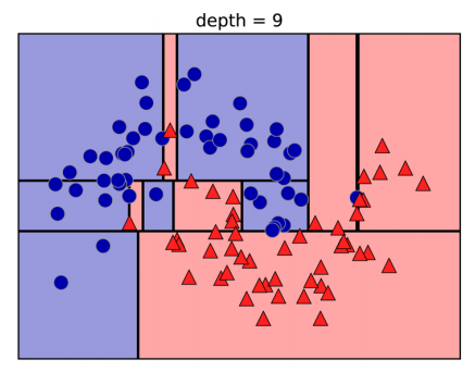
Typically, building a tree as described here and continuing until all leaves are terminal leads to models that are very complex and highly overfit to the training data. The presence of terminal leaves mean that a tree is 100% accurate on the training set; each data point in the training set is in a leaf that has the correct majority class.

The overfitting can be seen in the image above. You can see the regions determined to belong to class 1 in the middle of all the points belonging to class 0. On the other hand, there is a small strip predicted as class 0 around the point belonging to class 0 to the very right. This is not how one would imagine the decision boundary to look, and the decision boundary focuses a lot on single outlier points that are far away from the other points in that class.
There are two strategies to prevent overfitting
- stopping the creation of the tree early (also called pre-pruning)
- building the tree but then removing or collapsing nodes that contain little information (also called pos-pruning)
Possible criteria for pre-pruning include limiting the maximum depth of the tree, limiting the maximum number of leaves, or requiring a minimum number of points in a node to keep splitting it.
If we don’t restrict the depth of a decision tree, the tree can become arbitrarily deep and complex. Unpruned trees are therefore prone to overfitting and not generalizing well to new data.
Regression (Decision Trees vs Linear)
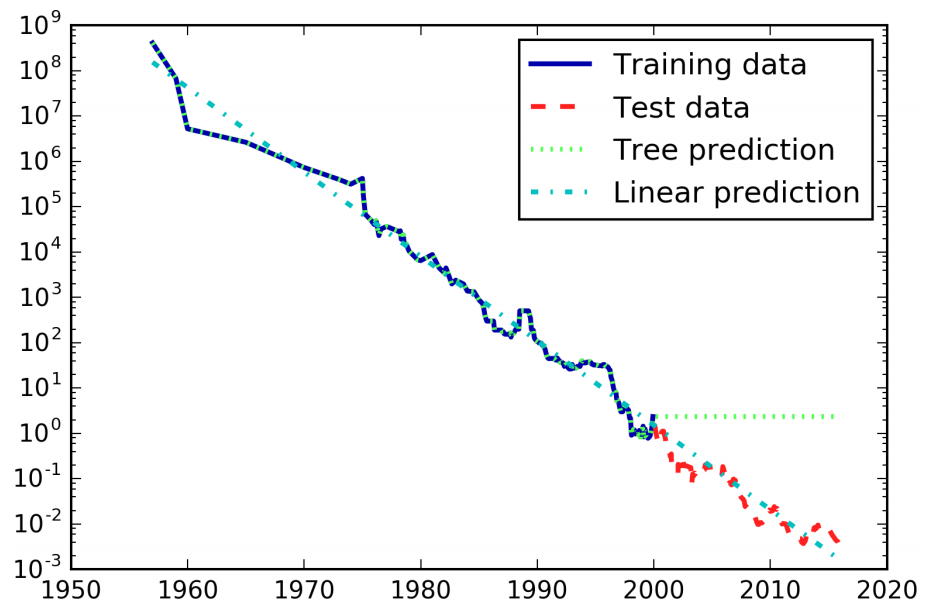
All that was said here on decision trees for classification is similarly true for decision trees for regression. The usage and analysis of regression trees is very similar to that classification trees. However, there is a particular property that is important to point out, though. All the tree based regression models are not able to extrapolate, or make predictions outside of the range of the training data.

The difference between the models is quite striking. The linear model approximates the data with a line, as we knew it would. This line provides quite a good forecast for the test data (the years after 2000), while glossing over some of the finer variations in both the training and the test data. The tree model, on the other hand, makes perfect predictions on the training data; we did not restrict the complexity of the tree, so it learned the whole dataset by heart. However, once we leave the data range for which the model has data, the model simply keeps predicting the last known point. The tree has no ability to generate “new” responses, outside of what was seen in the training data. This shortcoming applies to all models based on trees.
It is actually possible to make very good forecasts with tree-based models (for example, when trying to predict whether a price will go up or down). The point of this example was not to show that trees are a bad model for time series, but to illustrate a particular property of how trees make predictions.
Strenghts, Weaknesses, and Parameters
Decision trees have two advantages over many of the algorithms we’ve discussed so far: the resulting model can easily be visualized and undersood by nonexperts (at least for small trees), and the algorithms are completely invariant to scalling of the data. As each feature is processed separately, and the possible splits of the data don’t depend on scaling, no preprocessing like normalization or standarization of features is needed for decision tree algorithms. In particular, decision trees work well when you have features that are completely different scales, or a mix of binary and continuous features.
The main downside of decision trees is that even with the use of pre-pruning, they tend to overfit and provide poor generalization performance. Therefore, in most applications, the ensemble methods are usually used in place of a single decision tree.
Ensembles of Decision Trees
Ensembles are methods that combine multiple machine learning models to create a more powerful models. There are many models in the machine learning literature that belong to this category, but there are two ensemble models that have proven to be effective on a wide range of datasets for classification and regression, both of which use decision trees as their atomic modules: random forests and gradient boosted trees.