Linear Models

Linear models make a prediction using a linear function of the input features.

Linear Models for Regression

For regression, the general prediction for a linear model looks as follows:

Here, \(x_0\) to \(x_p\) denotes the features (in this example, the number of features is p) of a single data point, \(\Theta\) are parameters of the model that are learned, and \(y\) is the prediction the model makes.

Linear models for regression can be characterized as regression models for which the prediction is a line for a single feature, a plane when using two features, or a hyperplane in a higher dimensions.

For datasets with many features, linear models can be very powerful. In particular, if you have more features thain training data points, any target y can be perfectly modeled (on the training set) as a linear function.

There are many different linear models for regression. The difference between these models lies in how the models parameters \(\Theta\) are learned from the training data, and how model complexity can be controlled.

Linear Models for Classification

The formula looks very similar to the one for linear regression, but instead of returning the weighted sum of features, we threshold the predicted value at zero. If the function is smaller than zero, we predict the class -1; if it is larger than zero, we predict the class +1. The prediction rule is common to linear models for classification. Again, there are many different ways to find the coefficients \(\Theta\) and the intercept \(\Theta_0\).

For linear models for regression, the output, \(y\), is a linear function of the features: a line, plane, or hyperplane. For linear models for classification, the decision boundary is a linear function of the input. In other words, a (binary) linear classifier is a classifier that separates two classes using a line, a plane or a hyperplane.

The two most common linear classification algorithms are Logistic Regression and Linear Support Vector Machine.

The two models come up with similar decision boundaries. By default, both models apply an L2 regularization, in the same way that Ridge does for regression.

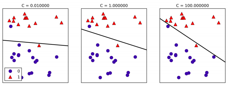
For Logistic Regression and Linear SVM the trade-off parameter that determines the strength of the regularization is called C, and higher values of C correspond to less regularization. In other words, when you use a high value of C, Logistic Regression and Linear SVM try to fit the training set as best as possible, while with low values of the parameter C, the models put more emphasis on finding a coefficient vector \(\Theta\) that is close to zero.

Another interessant aspect is how the parameter C acts. Using low values of C will cause the algorithms to try adjust to the “majority” of data points, while using a higher value of C stresses the importance that each individual data point be classified correctly.

Similarly to the case of regression, linear models for classification might seem very restrictive in low-dimensional spaces, only allowing for decision boundaries that are straight lines or planes. Again, in high dimensions, linear models for classification become very powerful, and guarding against overfitting becomes increasingly important when considering more features.

In:
from sklearn.datasets import load_breast_cancer

cancer = load_breast_cancer()
X_train, X_test, y_train, y_test = train_test_split(cancer.data, cancer.target stratify=cancer.target, random_state=42)

logreg = LogisticRegression().fit(X_train, y_train)
print("Training set score: {:.3f}".format(logreg.score(X_train, y_train)))
print("Test set score: {:.3f}".format(logreg.score(X_test, y_test)))

Out:
Training set score: 0.953
Test set score: 0.958

The default value of \(C=1\) provides quite good performance, with \(95\%\) accuracy on both the training and the test set. But as training and test set performance are very close, it is likely that we are underfitting. Let’s try to increase C to fit a more flexible model:

In:
logreg100 = LogisticRegression(C=100).fit(X_train, y_train)
print("Training set score: {:.3f}".format(logreg100.score(X_train, y_train)))
print("Test set score: {:.3f}".format(logreg100.score(X_test, y_test)))

Out:
Training set score: 0.972
Test set score: 0.965

Using \(C=100\) results in higher training set accuracy, and also a slightly increased test set accuracy, confirming our intuition that a more complex model should perform better. We can also investigate what happens if we use an even more regularized model than the default of \(C=1\), by setting \(C=0.01\):

In:
logreg001 = LogisticRegression(C=0.01).fit(X_train, y_train)
print("Training set score: {:.3f}".format(logreg001.score(X_train, y_train)))
print("Test set score: {:.3f}".format(logreg001.score(X_test, y_test)))

Out:
Training set score: 0.934
Test set score: 0.930

As expected, when moving more to the left along the scale from an already underfit model, both training and test set accuracy decrease relative to the default parameters.

Linear Models for Multiclass Classification

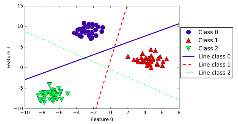
A common technique to extend a binary classification algorithm to a multiclass classification algorithm is the one-vs.-rest approach. In the one-vs.-rest approach, a binary model is learned for each class that tries to separate that class from all of the other classes, resulting in as many binary models as there are classes. To make a prediction, all binary classifiers are run on a test point. The classifier that has the highest score on its single class “wins, ” and this class label is returned as the prediction. Let’s visualize the lines given by the three binary classifiers

You can see that all the points belonging to class 0 in the training data are above the line corresponding to class 0, which means they are on the “class 0” side of this binary classifier. The points in class 0 are above the line corresponding to class 2, which means they are classified as “rest” by the binary classifier for class 2. The points belonging to class 0 are to the left of the line corresponding to class 1, which means the binary classifier for class 1 also classifies them as “rest.” Therefore, any point in this area will be classified as class 0 by the final classifier (the result of the classifica‐ tion confidence formula for classifier 0 is greater than zero, while it is smaller than zero for the other two classes).

But what about the triangle in the middle of the plot? All three binary classifiers classify points there as “rest”. Which class would a point there be assigned to? The answer is the one with the highest value for the classification formula: the class of the closest line.

Strenghts, Weaknesses, and Parameters

The main parameter of linear models is the regularization parameter, called alpha in the regression models and C in Linear SVM and Logistic Regression. Large values for alpha or small values for C mean simple models. In particular for the regression models, tunning these parameters is quite important. Usually C and alpha are searched for on a logarithmic scale. The other decision importante to make is whetever you want to use L1 regularization or L2 regularization. If you assume that only a few of your features are actually important, you should use L1. Otherwise, you should default to L2. L1 is actually important if interpretability of the model is important. As L1 will use only a few features, it is easier to explain which features are important to the model, and what features of these features are.

Linear features are very fast to train, and also fast to predict. They scale to very large datasets and work well with sparse data. If your data consists of hundreds of thousands or millions of samples, you might want to investigate using the \(solver = 'sag'\) option in Logistic Regression and Ridge, which can be faster than the default on large datasets.

Other options are the SGDClassifier class and the SGDRegressor class, which implement even more scalable versions of the linear models described here.

Another stregth of linear models is that they make it relatively easy to understand how a prediction is made, using the formulas we saw earlier for regression and classification. Unfortunally, it is often not entirely clear why coefficients are the way they are. This is particularly true if your dataset has highly correlated features; in these cases, the coefficients might be hard to interpret.

Linear models often perform well when the number of features is large compared to the number of samples. They are also often used on very large datasets, simply because it’s not feasible to train other models. However, in lower-dimensional spaces, other models might be yield better generalization performance.